|
1.1 Overview
iODA, short for integrative Omics Data Analysis, is user-friendly Java based graphical interface software. It implements an integrative platform for selection of statistical methods for heterogeneous data and performing different algorithms to detect differentially expressed genes. Then users can perform the pathway enrichment analysis based on human KEGG pathways (http://www.genome.jp/kegg). The differentially expressed genes can be obtained by 3 kinds of omics data; i.e mRNA, microRNA and ChIP-Seq data. All the panels and functions integrated in iODA can be used individually to tackle the analysis process. Compared to other software based on integrative analysis, iODA is the first local, algorithm selection, cross-multiple level of datasets, pathway enrichment analysis and easy to use software in one integrative platform. Then we make a consistency analysis on the results by an overlapping analysis.
We proposed six algorithms for heterogeneous detection incorporated in iODA are the list below.
●T-test - A t-test is any statistical hypothesis test in which the test statistic follows a Student's t distribution if the null hypothesis is supported. It can be used to determine if two sets of data are significantly different from each other, and is most commonly applied when the test statistic would follow a normal distribution if the value of a scaling term in the test statistic were known.
Recently, it has been recognized that many oncogenes show altered expression in only a small proportion of cancer samples(Lian, 2008). Such features will be removed when using t-test or t-test like methods because they average gene expression levels in all the studied samples. Tomlin et al. conclude that t-tests were not adequate for detecting heterogeneous patterns of oncogenes (Tomlins, et al., 2005).
●LSOSS - LSOSS is the abbreviation of Least Sum of Ordered Subset Squared, The general idea of LSOSS is to use the sum of squares of two ordered subsets of cancer samples to estimate the square sum of the t-statistic and to use the mean value of the appealing subset of cancer samples to estimate the mean value of cancer samples of the t-statistic(Wang and Rekaya, 2010).
●MOST - MOST is the abbreviation of maximum ordered subset t-statistics, Lian et al proposed another statistics for the detection of cancer differential gene expression which have similar power to ORT when the number of activated samples is very small, but perform better when more samples are differentially expressed(Lian, 2008).
●COPA - Tomlins et al (2005) have proposed the "cancer outlier profile analysis" (COPA) method for detecting cancer genes which show increased expressions in a subset of disease samples. They argue that in the majority of cancer types, oncogene has heterogeneous activation patterns; traditional analytical methods, for example, t-statistic, which search for common activation of genes across a class of cancer samples, will fail to find such oncogene expression profiles(Wu, 2007).
●ORT - Wu et al study statistical methods to detect cancer genes that are over- or down-expressed in some but not all samples in a disease group. This has proven useful in cancer studies where oncogenes are activated only in a small subset of samples. They propose the outlier robust t-statistic (ORT), which is intuitively motivated from the t-statistic; the most commonly used differential gene expression detection method(Wu, 2007).
●OS - Tibshirani et al proposed a method for detecting genes that, in a disease group, exhibit unusually high gene expression in some but not all samples. This can be particularly useful in cancer studies, where mutations that can amplify or turn off gene expression often occur in only a minority of samples.
We propose three different omics level data which can be analyzed in iODA are the list below:
1.Gene expression data (mRNA level)
2.MicroRNA level data
3.ChIP-Seq level data
iODA provide a novel platform with emphasis on the pathways consistency analysis generated from pathway enrichment analysis from multiple omics data, which will finally lead to a robust pathway list. This software is particularly useful for researchers who want to integrate different level omics data and various datasets from different researchers for further pathway enrichment analysis and make a consistency analysis on the pathway results. We have verified the hypothesis that common molecular signatures are more similar at the pathway level than at the gene level. So we propose this platform to eliminate the heterogeneity of different datasets and integrative the different omics datasets at a system level and obtain deeper insight on the underlying biological mechanisms of the data generated from gene microarrays, microRNA microarrays and next generation sequencing ChIP-Seq data.
With the application of software iODA, biologists will find it easy to analyze the omics data from different omics levels and datasets with pathway enrichment analysis. The whole workflow for each dataset analysis was integrated in iODA, such as test for best algorithm to perform outlier detection, differentially expressed genes detection by appropriate algorithm, differentially expressed microRNAs detection by appropriate algorithm, microRNAs target genes detection, ChIP-Seq data peaks detection, KEGG pathway enrichment analysis, pathway consistency analysis with different omics level.
This tutorial helps users to run iODA on Linux (Ubuntu for example) and Windows (7 or later versions) to facilitate the biological data interpretation in a step-by-step style.
1.2 Basic concepts
1.2.1 Pathway
A pathway is a group of related, genes, metabolites, and their mutual interactions, which form an aggregate biological function. A similar concept is gene/compound set, which means some manually defined gene/compound sets according to their functionality or ontology. Gene/compound set can be interpreted as a superior concept of pathway.
The KEGG pathway map is a molecular interaction/reaction network diagram represented in terms of the KEGG Orthology (KO) groups, so that experimental evidence in specific organisms can be generalized to other organisms through genomic information. Each map is manually drawn with in-house software called KegSketch, which generates the KGML+ file. This file is an SVG file containing graphics objects that are associated with KEGG objects.
1.2.2 Gene expression data
Gene expression is the process by which information from a gene is used in the synthesis of a functional gene product. In genetics, gene expression is the most fundamental level at which the genotype gives rise to the phenotype. The genetic code stored in DNA is "interpreted" by gene expression, and the properties of the expression give rise to the organism's phenotype. Such phenotypes are often expressed by the synthesis of proteins that control the organism's shape, or that act as enzymes catalyzing specific metabolic pathways characterizing the organism.
Publicly available microarray expression datasets can be downloaded by Gene Expression Omnibus (http://www.ncbi.nlm.nih.gov/geo/) database which had been generated by independent laboratory. These datasets were measured with different technologies and platforms. Comparative cancer analyses included cancer versus respective normal tissue, high grade versus low grade cancer, poor outcome versus good outcome, metastatic versus primary cancer, and subtype1 versus subtype2. Thus, our analysis across multiple datasets, based on normal prostate versus tumor prostate samples, was comparable.
1.2.3 MicroRNA data
MicroRNAs (miRNAs) are small non-coding RNAs of approximately 22-nucleotides. They play important roles in gene regulation at post-transcriptional level. They are able to repress the activity of complementary mRNAs by targeting the 3’-untranslated regions(Bartel, 2009). Release 19 of the miRBase database contains more than 2200 mature miRNA sequences for human(Kozomara and Griffiths-Jones, 2011). Aberrant miRNA expression was shown related to the generation of cancer stem cells and the tumor genesis(Lin, et al., 2010; Liu, et al., 2011; Mallick, et al., 2011). Microarray-based technologies have routinely been used for profiling molecular expression in cancer. Microarray allows simultaneous expression profiling of tens of thousands of genes in normal versus malignant cells. We can use these miRNA microarray datasets to detect the differentially expressed miRNAs. Then we obtain the target genes of them.
1.2.4 ChIP-Seq data
The disease associated ChIP-Seq datasets were extracted from Gene Expression Omnibus (GEO). Peak detection algorithm is crucial to the analysis of ChIP-Seq dataset(Ding, et al., 2012). Currently, several tools are available to identify genome-wide binding sites of transcription factors, such as FindPeaks(Fejes, et al., 2008), F-Seq (Boyle, et al., 2008), CisGenome(Ji, et al., 2011), MACS (Zhang, et al., 2008), SISSRs (Narlikar and Jothi, 2012), and QuEST (Valouev, et al., 2008). These different methods have their own advantages and disadvantages, although they act in a similar manner. ChIP-Seq data has regional biases because of sequencing and mapping biases, chromatin structure, and genome copy number variations (Redon, et al., 2006). In order to get more stable result, the iODA integrate MACS tool to identify the binding sites of disease related transcription factors in this study. The tool uses control samples to guide peak finding and calculate the FDR (False Discovery Rate) value of peaks. Then iODA also provide the PeakAnalyzer tool to annotate the peaks.
1.2.5 Pathway enrichment analysis
Pathway Enrichment Analysis is the analysis to find the most relevant pathway, according to the gene/protein data, by calculating their differentially expression (DE) values to fit in an enrichment model, and finally returns a list of pathways ranked by certain enrichment score. Currently, most evaluations of enrichment score employ probability approach, such as p-value.
Pathway enrichment analysis helps reveal the underlying biological pathway/function from large biological data. It is the most commonly used in-silico function analysis for high-throughput omics data.
In iODA, KEGG, an open access database resource, was selected for pathway enrichment analysis. Both “Local pathway enrichment” and “Online pathway enrichment” functions were designed. The former utilizes the local KEGG database and calculates p-values through hypergeometric distribution algorithm, whereas the latter uses HTTP protocol to submit a request to the KEGG web server and receives the pathway results. Here the local pathway database needs to be periodically updated and the online function requires an internet connection, so the response time is based on the status of network and the KEGG server. After submitting the dysfunctional gene list, the returning result contains information of enriched pathway ID, pathway symbol, the number of submitted genes in this pathway, the number of all genes in this pathway, p-value, q-value and DE-gene list.
1.3 Pipeline
iODA guides users to follow the pipeline, i.e., selection of statistical methods for heterogeneous data, expression data input, detect the differentially expressed outliers with the selected algorithm, microRNA target genes detection, ChIP-Seq data annotation, pathway enrichment analysis, cross mapping and consistency analysis to perform meta-analysis on pathway results, (Figure 1).
In this study, iODA integrative three different levels of omics data and make a meta-analysis on the pathway results. For each omics level, there are a few datasets from the different laboratories, thus we make a consistency analysis on pathway level to get the common pathway results. Then we make a meta-analysis for all three omics level results.
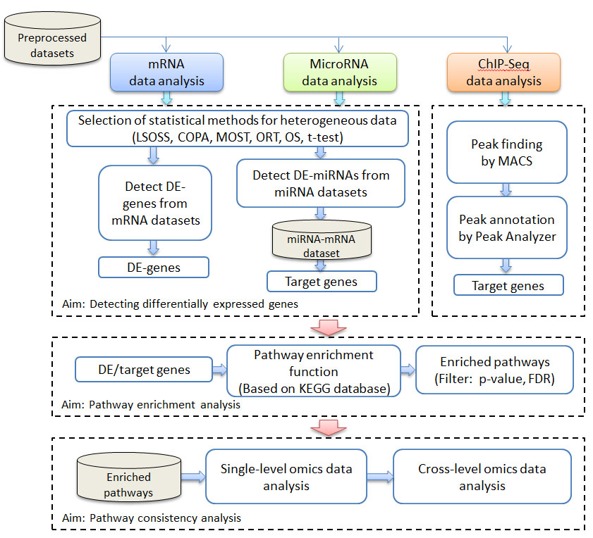
Fig. 1. The working pipeline of iODA. It provides the function of DE-gene/miRNA identification, pathway enrichment and consistency analysis.
| Chapter 2 Installing iODA |
2.1 Downloading iODA
iODA can be downloaded from home page under GPL version3.
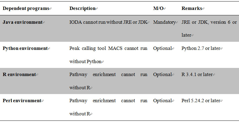
The dependent programs of iODA are Java, Python, R, Perl (available in their official websites).
Table 1 The dependent programs of iODA
2.2 Installing iODA
iODA itself is a Java based program which needs No installation and can be run on Linux (Ubuntu for example) and Windows (7 or later versions). To run iODA Java, R, Perl environment must be installed. If users want to use ChIP-Seq level data analysis, they need install the Python environment.
2.2.1 Java environment installation
For Linux, users should install the "Java SE Development Kit" in the terminal and proceed. For example, in Ubuntu type "sudo apt-get install oracle-java7-installer" in the terminal. For Windows, you can download the binary installer from the website (http://www.oracle.com/technetwork/java/javase/downloads/index.html). Using Windows, users need to open up the system properties dialog, and locate the tab labeled Environment. Add your Java path to the PATH variable.
2.2.2 R environment installation
For Linux, users should download and install the R environment in the terminal and proceed. For example, in Ubuntu type "apt-get install r-base" in the terminal.
For Windows, you can download the binary installer from the website (https://www.r-project.org/). Using Windows, users need to open up the system properties dialog, and locate the tab labeled Environment. Add your R path to the PATH variable.
2.2.3 Perl environment installation
For Linux, users should download and install the Perl environment in the terminal and proceed. For example, in Ubuntu type "apt-get install perl " in the terminal.
For Windows, you can download the binary installer from the website (http://www.perl.org/). Using Windows, users need to open up the system properties dialog, and locate the tab labeled Environment. Add your Perl path to the PATH variable.
2.2.4 Python environment installation
If users want to make the ChIP-Seq level data analysis, MACS should be run in this panel as Python environment should be installed. For example, in Ubuntu type "apt-get install python2.7" in the terminal.
For Windows, you can download the binary installer from the website (https://www.python.org/). Using Windows, users need to open up the system properties dialog, and locate the tab labeled Environment. Add your Python path to the PATH variable.
3.1 Running iODA
iODA can run under Windows and Linux. First, users open the iODA folder and then double click the "IntegrativeOmicsDataAnalysis.jar" file to run the software. The main interface of iODA (figure 2) will appear if everything goes well.
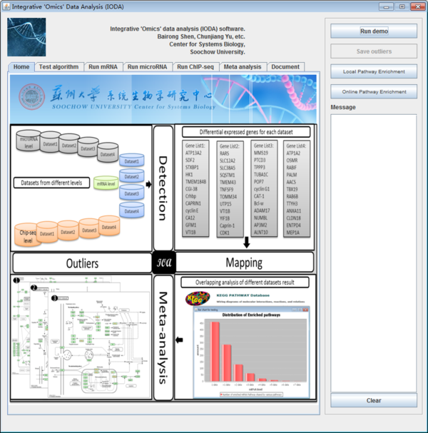
Fig. 2. The main interface of iODA.
3.2 Function Panels
After installation, iODA show a homepage of the software, there are six panels which conclude the different sub panels as shown below.

Fig. 3. The function panels of iODA.
Each panel means different function. Users can select the different panels by click the tabbed navigation.
| Chapter 4 The first step - Selection of statistical methods for heterogeneous data |
iODA contains Test algorithm panel, if users click the "Test algorithm" panel, they can use this function as shown below.
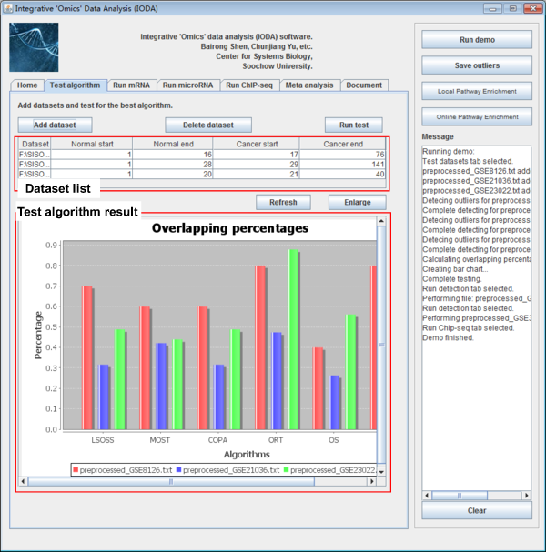
Fig. 4. The Test algorithm panel of iODA.
4.1 Input datasets
This panel is designed for mRNA/miRNA level microarray expression data. To address the complexity that t-tests were not adequate for detecting heterogeneous patterns of oncogenes. iODA compares the performance of the six methods in obtaining the disease associated DE-mRNAs and DE-miRNAs. We considered the DE-mRNAs and DE-miRNAs detected by at least four methods to be putative outliers. The percentage of these putative outliers in the original result of each method was calculated to measure the method’s accuracy.
Users can choose the algorithm performs better than the other methods which has the biggest median observation and smallest standard deviation. Then users can take the result by the best algorithm for the downstream analyses.
4.1.1 mRNA (gene expression) data
Users can input mRNA microarray datasets to test the best algorithm. Here, all the dataset for algorithm detection must be imported with the same omics level. All the data should be prepared in the uniform plain text containing pre-processed expression of all samples. The demo data is described in 10.1.
4.1.2 MicroRNA data
Users can input microRNA microarray datasets to test the best algorithm. Here, all the dataset for algorithm detection must be imported with the same omics level. All the data should be prepared in the uniform plain text containing pre-processed expression of all samples. The demo data is described in 10.2.
4.2 Process for detecting outliers
After preparing the mRNA and microRNA expression datasets, users need to add expression datasets to the datasets list table. After clicking the button "Add dataset" a new window will be popped up, users should input files which are prepared as the specified format. And the datasets should be prepared in the same omics level. Users click the button "Browse", then typing where the normal and malignant samples start and end. Finally the dataset will be loaded to the dataset list table after clicking the button "OK". Users should be cautious to the start and end columns of samples.
The datasets list table will list the file path of each dataset and where the normal start and end and the cancer start and end. Users can edit the start and end number in the table if it is needed. Users can delete the datasets by clicking the button "Delete dataset" if users get it wrong with sample classification sometimes and reset the table by clicking the button "Reset".
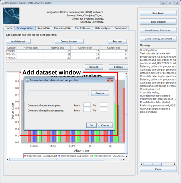
Fig. 5. The interface after clicking the "Add dataset" button
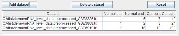
Fig. 6. The dataset list after three datasets are added.
4.3 Selection of statistical methods
After importing the test datasets, users click the button "Run test" to test for the best algorithm. A bar chart of the result will give an indicative of the best algorithm selection. An example of bar chart shows below. The different color means different dataset, the Y-axis means the percentage of the putative outliers in each dataset.
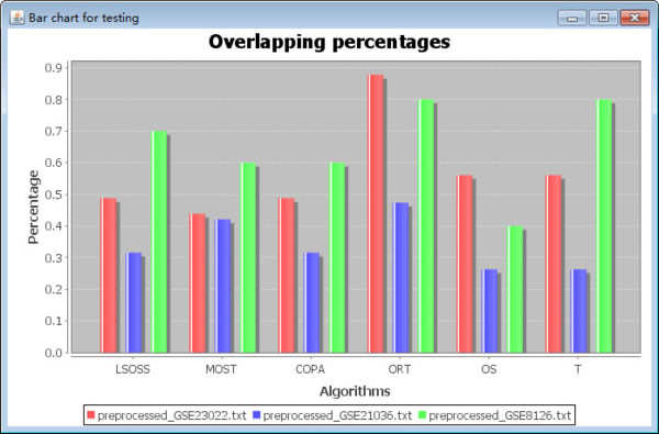
Fig. 7. Overlapping percentages of putative outliers. The different colors signify different datasets, the X-axis represents the six algorithms, and the Y-axis indicates the percentage of the putative outliers in each dataset.
The putative outlier percentages are calculated as follows:
1. Detecting the outliers of each dataset using the six algorithms (termed as Oi, 1=< i <=6);
2. Counting the number of occurrences of each outlier in the six outlier results from step 1;
3. Screening the outliers with number of occurrences no fewer than four (termed as OF);
4. The accuracy percentage is calculated as OF / Oi (1=< i <=6)
| Chapter 5 The second step - Pathway enrichment analysis |
iODA can obtain differentially expressed outliers and users can map them to the pathway enrichment tool by themself. There are many functional annotation systems which can be used to perform the pathway enrichment analysis for gene function, such as Gene Ontology (GO) categories(Ashburner, et al., 2000), canonical KEGG Pathway Maps(Kanehisa and Goto, 2000), and commercial software MetaCore-GeneGo Pathway Maps.
KEGG Mapper – Search Pathway is the basic pathway mapping tool, where given objects (genes, proteins, compounds, glycans, reactions, drugs, etc.) are searched against KEGG pathway maps and found objects are marked in red. The objects in different types of pathway maps are specified by the following KEGG identifiers and aliases.
This data is last updated on June 10, 2014.
Table 2 KEGG identifiers and aliases
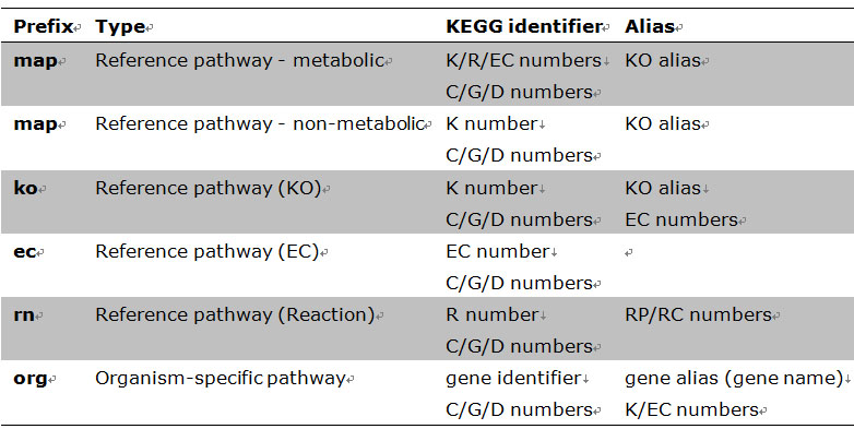
In order to provide convenience for users, we also integrate the KEGG mapping tool in the iODA. The differentially expressed genes can be input as objects, and users will get the enriched pathway results.
For iODA, in each omics type data analysis, there are "Local pathway enrichment" and "Online pathway enrichment" button which can be used to perform the pathway enrichment analysis in the right panel as shown below.
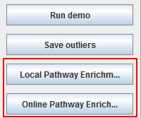
Fig. 8. The pathway enrichment buttons.
5.1 Local pathway enrichment
After clicking the "Local pathway enrichment" button, a new window will be popped up. We made a Java based GUI for KEGG pathway enrichment and integrate it in iODA. Local pathway enrichment uses local pathways data we downloaded from KEGG. The data is saved at iODA\lib\KEGGPathway\ new.hsa.kegg.xls. Users can update it if needed. We recommend users use this to do KEGG enrichment analysis.
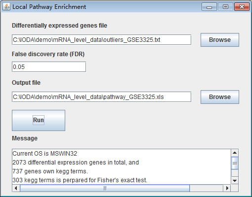
Fig. 9. The local pathway enrichment interface.
The steps of using local pathway enrichment to do pathway enrichment are as follows.
Step 1: Input differentially expressed genes file
Click the "Browse" button to select the differentially expressed genes file.
Step 2: Input false discovery rate
Input the FDR value. The enriched pathway result will be filtered by this value. If input value is 1 then the entire enriched pathway will be returned.
Step 3: Input output file
Click the "Browse" button to select the output file. We recommend use "xls" as the file extension.
Step 4: Click run button
The result contains information about pathway ID, pathway symbol, differentially expressed genes in this pathway, all genes in this pathway, p-value, q-value and differentially expressed gene list.
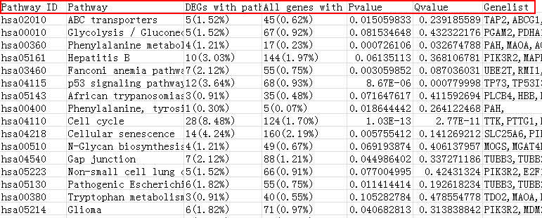
Fig. 10. The local pathway enrichment result.
5.2 Online pathway enrichment
After clicking the "Online pathway enrichment" button, a new window will be popped up. We made a Java based GUI for KEGG pathway enrichment and integrate it in iODA. Online pathway enrichment uses HTTP protocol to submit request to KEGG server and receive response. It needs the computer connect to internet and the response time is based on the network status and the KEGG server.
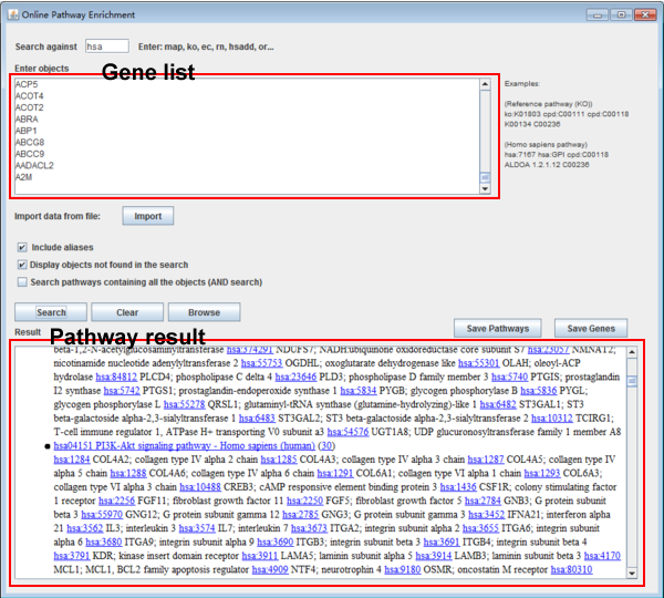
Fig. 11. The online pathway enrichment interface.
The steps of using online pathway enrichment to do pathway enrichment are as follows.
Step 1: Input the objects
Users need to input the different expressed genes in the "enter objects" textbox. Users can also import the different expressed genes from file.
Step 2: Set the parameters
Users can set the different parameters in the following in the check box. Users can include the aliases for each object, and display the objects which are not found in the given list. Moreover, users can also search pathways containing all objects.
Step 3: Save the results
After clicking the search button, the pathway results will be emerged in the "result" textbox, users can save the Pathway and Gene results by clicking the "Save Pathways" and "Save Genes" button. Then the results will be stored in text file with the pathway and enriched gene information. There is an example result file shown below. The result contains pathways and their enriched genes.
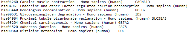
Fig. 12. The online pathway enrichment result.
| Chapter 6 The third step-Run mRNA level |
Users can make the mRNA (gene expression) analysis after chose the "Run mRNA" panel. The panel is shown below.
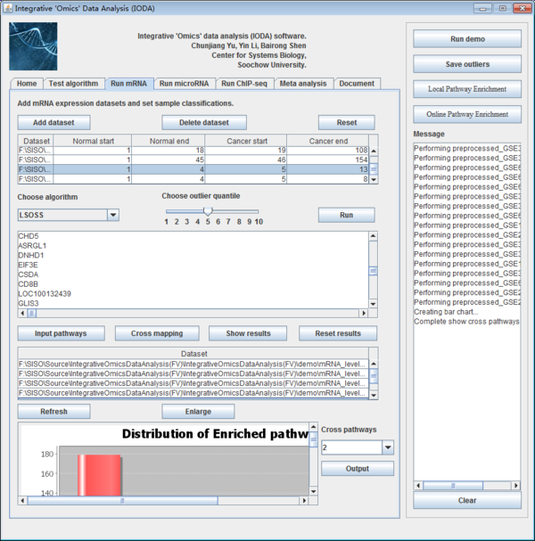
Fig. 13. The interface of run mRNA panel.
6.1 Prepare mRNA expression datasets
Firstly, users need to prepare the mRNA expression data to the requirement of iODA for the following analysis.
Uniform plain text containing pre-processed expression of all samples:
●Tab/comma delaminated
●One head row and one ID column
●Equal columns each row
●Pre-processed
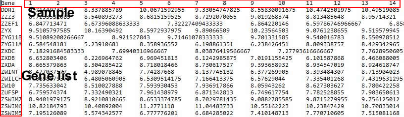
Fig. 14. The pre-processed mRNA expression data.
6.2 Add mRNA expression datasets to dataset list table
After preparing the mRNA level expression datasets, users need to add mRNA expression datasets. After clicking the button "Add dataset", then a new window will be popped up, users should input file which are prepared as the specified format. Users click the button "Browse", then typing where the normal and malignant samples start and end. Finally the dataset will be loaded to the datasets list table after clicking the button "OK". Users should be cautious to the start and end columns of samples.
The datasets list table will list the file path of each dataset and where the normal start and end and the cancer start and end. Users can edit the start and end number in the table if it is needed. Users can delete the datasets by clicking the button "Delete dataset" if users get it wrong with sample classification sometimes and reset the table by clicking the button "Reset".
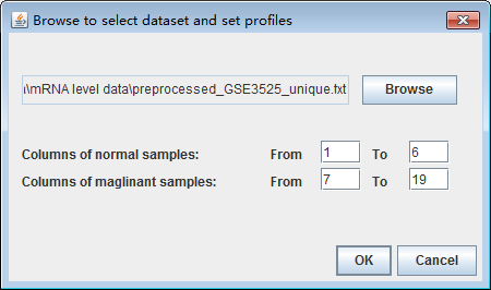
Fig. 15. The interface after clicking the "Add dataset" button
6.3 Identification of differentially expressed genes
After importing the various datasets users choose the appropriate algorithm to deal with the input datasets. This panel also provides the different outlier quantile to obtain the different results which make a limit of quantity. By choosing algorithm and outlier quantile, then users click the button "Run" to make the differentially expressed genes identification. The results will be shown in the follow textbox and click the button "Save outliers" in the right panel to save the results with the dataset name.
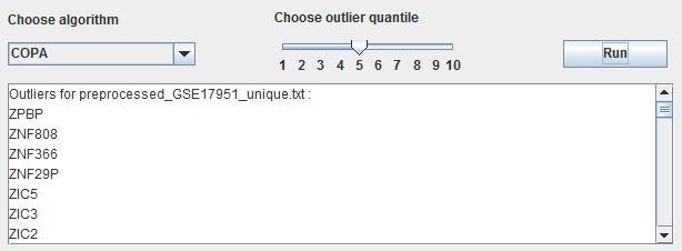
Fig. 16. The result of identification of differentially expressed genes.
6.4 Pathway enrichment analysis
With the outlier genes, users can input the gene objects and got the pathways results as shown in Chapter 5.
6.5 Pathways cross mapping
Meanwhile, users can input the enriched pathway results and make the consistency analysis. Users click the button "Input Pathways" to import the enriched pathways. Then the file path will be shown in the follow table. After selecting the pathway files users can see the overlapping results by clicking the button "Cross mapping". Then the overlapping pathway results will be shown in the text box upon the pathways list table. The results will show the pathway name, the times it appears and the genes in the pathway.
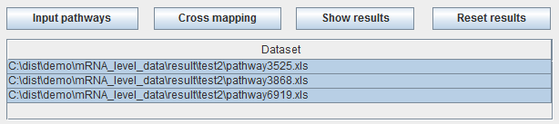
Fig. 17. The pathway list table.
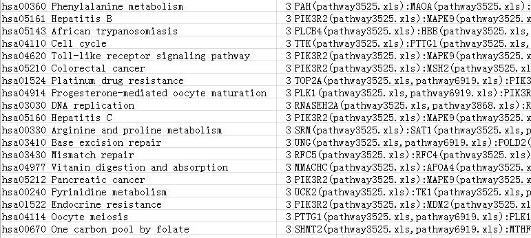
Fig. 18. The result of pathways cross mapping.
6.6 Show pathway cross mapping results
Users click the button "Show results" to see the pathway results in the panel. We make a bar chart by the various pathway results which will be shown in the box. A distribution of enriched pathways is shown in a bar chart. The box is not enough to show all bar graph, users can click the button "Enlarge". There will be a new window to show the results. The y-axis is the amount of the enrich pathways appear in how many datasets while the x-axis is the frequency of the data occurrence in various datasets. ">=1 data" means the enriched pathways appear how many times. The bar graph is made to show the enriched pathways clearly; afterwards users will make the consistency analysis by select the pathways which are appearing in the appropriate datasets in the combo box in the right of bar graph panel. The number means the appearance times. Later, users click the button "Output" to output the results. Moreover, users can clear the text box by clicking the button "Reset results".
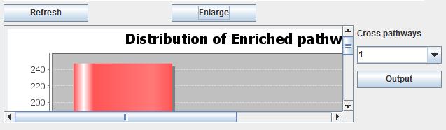
Fig. 19. The bar chart of pathway cross mapping result.
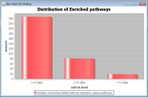
Fig. 20. The enlarged bar chart.
Then the output file will include some information about the pathway as shown below:
1.Pathway name
2.Pathway occurrence count
3.The enriched genes in each pathway
4.The enriched genes belong to which dataset
Finally, the whole steps were completed here. First of all, users should prepare the mRNA expression data, and then identify the differentially expressed genes by choosing the appropriate algorithm and outlier quantile. Secondly, the detected genes are mapped to KEGG pathway which are integrated in iODA to make the pathway enrichment analysis. Thirdly, the consistency analysis was applied on the pathway results.
| Chapter 7 The forth step-Run microRNA level |
Users can make the microRNA level analysis after choosing the "Run microRNA" panel. The panel is shown below.
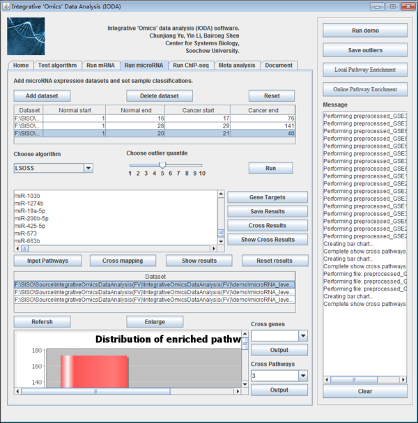
Fig. 21. The interface of run microRNA panel.
7.1 Prepare microRNA expression datasets
Firstly, users need to prepare the microRNA expression to the specified format of iODA for the following analysis.
Uniform plain text containing pre-processed expression of all samples:
●Tab/comma delaminated
●One head row and one ID column
●Equal columns each row
●Pre-processed
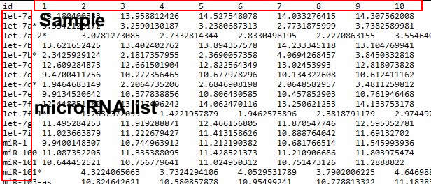
Fig. 22. The pre-processed microRNA expression data.
7.2 Add microRNA expression datasets to dataset list table
It is the same as shown in the mRNA level. Please reference step 2 of chapter 6.
7.3 Identification of differentially expressed microRNAs
After importing the various datasets users choose the appropriate algorithm to deal with the input datasets. This panel also provides the different outlier quantile to obtain the different results which make a limit of quantity. By choosing algorithm and outlier quantile, then users click the button "Run" to make the differentially expressed genes identification. The results will be shown in the follow textbox and click the button "Save outliers" in the right panel to save the results with the dataset name. It is also same as shown in the mRNA panel.
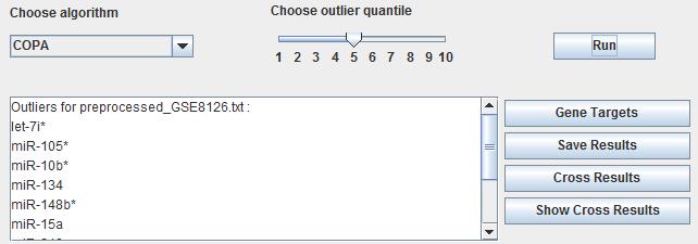
Fig. 23. The result of identification of differentially expressed microRNA.
7.4 MicroRNA target genes detection
After generating differentially expressed microRNAs users can get the target genes from the detected microRNAs by clicking the button "Gene targets" as shown below.
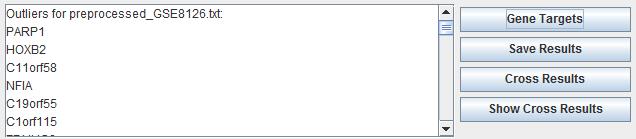
Fig. 24. The target genes of detected microRNAs.
iODA uses a integrative miRNA-mRNA targeting dataset which was the combination of experimentally validated targeting data and computational prediction data and has been proposed in our previous work (Zhang, et al.). The experimentally validated data consist of information from different databases, such as miRecords (Xiao, et al., 2009), TarBase (Sethupathy, et al., 2006), miR2Disease(Jiang, et al., 2009), and miRTarBase (Hsu, et al., 2011). Meanwhile, the computational prediction data comprised information from miRNA-mRNA target pairs residing in no fewer than 2 datasets from HOCTAR (Gennarino, et al., 2011), ExprTargetDB (Gamazon, et al., 2010), and starBase (Yang, et al., 2011). In total, there were 48868 regulation pairs among 618 miRNAs and 9526 target genes. The miRNA-mRNA targeting data is saved at iODA\ miRNA_mRNA_interaction_network.txt. Users can update it if needed.
7.5 Target genes cross mapping
The target genes are detected from various datasets. In order to obtain the enriched pathways results, there are two ways to obtain the differentially expressed genes.
On one hand, users can map the target genes from each microRNA dataset to KEGG pathway enrichment tool, respectively. Then users can get the consistency results as the same shown in mRNA level. On the other hand, users can make the gene consistency analysis before pathways enrichment analysis. It can identify the target genes involved in all datasets. The target genes which are targeted by most of microRNA datasets maybe play an important role in the cancer progression. At first, users click the button "Cross Results" to cross the results for each dataset, then the target genes appear times will be stored in the memory. Secondly, users click the button "Show Cross Result" to see the target genes overlapping results in gene level as shown below. The y-axis is the amount of genes appears in multiple datasets. And the x-axis is the target genes in how many datasets. The bar graph represents the distribution of enriched target genes. It is similar as shown in pathway consistency analysis. There are two choices in the right side of the bar chart box. Users can select the number of cross genes from the "Cross genes" combo box. The number is enriched target genes shared by number datasets. At last uses click the "Output" button to output the genes in various datasets.
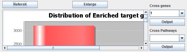
Fig. 25. The enriched target genes.
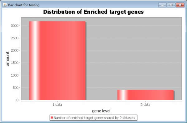
Fig. 26. The enlarged bar chart of enriched target genes.
7.6 Pathway enrichment analysis
With the outlier genes from the cross genes results or target genes from each dataset, users can got the pathway results as shown in Chapter 5.
7.7 Pathways cross mapping
Making the consistency analysis of enriched pathways, users can follow the same steps as shown in the step 5 in chapter 6.
7.8 Show pathway cross mapping results
Here, this step is same to the step 6 in chapter 6. Users can get the pathway overlapping results.
| Chapter 8 The fifth step-Run ChIP-Seq level |
The analysis of ChIP-Seq was integrated in the iODA in "Run ChIP-Seq" panel. The panel is shown below. There are also three sub tabs for the downstream analysis. It is MACS tool, PeakAnalyzer tool and Results.
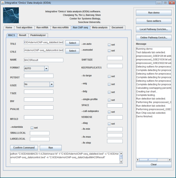
Fig. 27. The interface of run ChIP-Seq panel.
8.1 Prepare ChIP-Seq datasets
Firstly, users need to prepare the ChIP-Seq data to the requirement of iODA for the following analysis.
Here, users can use the ChIP-Seq datasets which are the binding sites of the disease related specific transcription factors, such as AR and FoxA1.
Uniform plain text should follow the note:
For BED format, the 6th column of strand information is required by MACS. And please pay attention that the coordinates in BED format is zero-based and half-open (http://genome.ucsc.edu/FAQ/FAQtracks#tracks1).
For plain ELAND format, only matches with match type U0, U1 or U2 is accepted by MACS, i.e. only the unique match for a sequence with less than 3 errors is involed in calculation. If multiple hits of a single tag are included in your raw ELAND file, please remove the redundancy to keep the best hit for that sequencing tag.
For the experiment with several replicates, it is recommended to concatenate several ChIP-Seq treatment files into a single file. To do this, under Unix/Mac or Cygwin (for windows OS), type:
$ cat replicate1.bed replicate2.bed replicate3.bed > all_replicates.bed
ELAND export format support sometimes may not work on your datasets, because people may mislabel the 11th and 12th column. MACS uses 11th column as the sequence name which should be the chromosome names.
We show an example of uniform file as below:
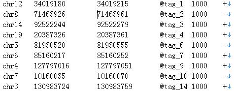
Fig. 28. An example of ChIP-Seq data.
8.2 Peak detection by MACS
Next generation parallel sequencing technologies made chromatin immunoprecipitation followed by sequencing (ChIP-Seq) a popular strategy to study genome-wide protein-DNA interactions, while creating challenges for analysis algorithms. Zhang et al present Model-based Analysis of ChIP-Seq (MACS) on short reads sequencers such as Genome Analyzer (Illumina / Solexa). MACS empirically models the length of the sequenced ChIP fragments, which tends to be shorter than sonication or library construction size estimates, and uses it to improve the spatial resolution of predicted binding sites. MACS also uses a dynamic Poisson distribution to effectively capture local biases in the genome sequence, allowing for more sensitive and robust prediction. MACS compares favorably to existing ChIP-Seq peak-finding algorithms, is publicly available open source, and can be used for ChIP-Seq with or without control samples(Zhang, et al., 2008).
To install the MACS tool, Python version must be equal to 2.6 or 2.7 to run it. We recommend using the version 2.7. The MACS tool provided by Zhang et al is based on command terminal. In order to make it convenient for users and integrated in iODA on Java platform, we make a visualization of MACS tool on Java platform instead of command line.
There are many options for users to set parameters in command line by MACS. Here, we make these parameters in a visual way and users can set and fill it by themselves easily. If users are used to run it on command line, they can also click the button "Create Command" to fill the command line in textbox. Here, we make the default parameter initially. Users can click the button "select" around the TFILE to input the ChIP-Seq data while clicking the button "select" around the CFILE to input the control data. Afterwards, users should iput the name of the output file in the textbox called "NAME". After setting the parameters, users will click the button "Run" to generate the peaks detection results.
Note: If you are interested on the details on the parameters, please visit the original website of MACS (http://liulab.dfci.harvard.edu/MACS/index.html).
There may be many different kinds of output files as follows:
NAME_peaks.xls is a tabular file which contains information about called peaks. You can open it in excel and sort/filter using excel functions. Information include: chromosome name, start position of peak, end position of peak, length of peak region, peak summit position related to the start position of peak region, number of tags in peak region, -10*log10 (pvalue) for the peak region (e.g. pvalue is 1e-10, then this value should be 100), fold enrichment for this region against random Poisson distribution with local lambda, FDR in percentage. Coordinates in XLS is 1-based which is different with BED format.
NAME_peaks.bed is BED format file which contains the peak locations. You can load it to UCSC genome browser or Affymetrix IGB software.
NAME_summits.bed is in BED format, which contains the peak summits locations for every peaks. The 5th column in this file is the summit height of fragment pileup. If you want to find the motifs at the binding sites, this file is recommended.
NAME_negative_peaks.xls is a tabular file which contains information about negative peaks. Negative peaks are called by swapping the ChIP-Seq and control channel.
NAME_model.r is an R script which you can use to produce a PDF image about the model based on your data. Load it to R by: $R --vanilla < NAME_model.r Then a pdf file NAME_model.pdf will be generated in your current directory. Note: R is required to draw this figure.
NAME_treat/control_afterfiting.wig.gz files in NAME_MACS_wiggle directory are wiggle format files which can be imported to UCSC genome browser/GMOD/Affy IGB. The .bdg.gz files are in bedGraph format which can also be imported to UCSC genome browser or be converted into even smaller bigWig files.
NAME_diag.xls is the diagnosis report. First column is for various fold_enrichment ranges; the second column is number of peaks for that fc range; after 3rd columns are the percentage of peaks covered after sampling 90%, 80%, 70% ... and 20% of the total tags.
NAME_peaks.subpeaks.bed is texts file which IS NOT in BED format. This file is generated by PeakSplitter (<http://www.ebi.ac.uk/bertone/software/PeakSplitter_Cpp_usage.txt>) when —call-subpeaks option is set.
Here, we show an example of NAME_peaks.bed file which is obtained by the demo files using MACS:
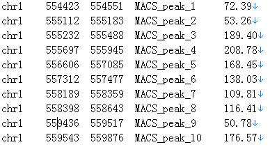
Fig. 29. An example of MACS result.
8.3 Peak annotation by PeakAnalyzer
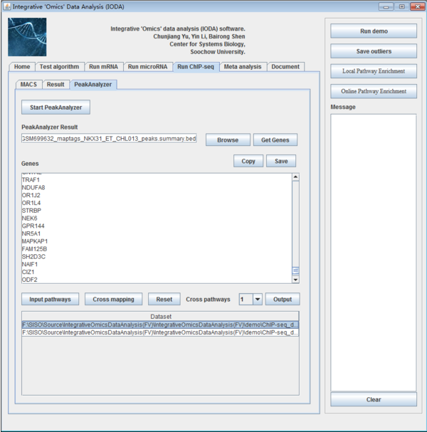
Fig. 30. The interface of PeakAnalyzer panel.
After obtaining the peaks detection results, in order to study these peaks in biological way, we need to understand the position of these peaks in the genome sequence and the containing genes nearby it. PeakAnalyzer is a free tool to achieve these functions in graphic user interface (GUI) which can be downloaded on the website (http://www.bioinformatics.org/peakanalyzer/wiki/Main/Download). Here, we also integrative it in iODA.
Turning to "PeakAnalyzer" tab, users can click the button "Start PeakAnalyzer" to run the PeakAnalyzer tool, a new window will be popped up as shown below.
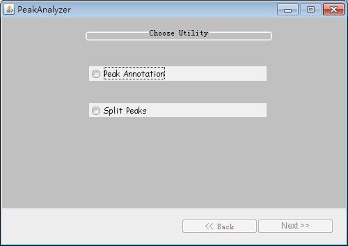
Fig. 31. The interface of PeakAnalyzer.
At first, there are two choices, here, we choose the "Peak Annotation" and click button "Next". Afterwards, there will be three choices called "NDG-Nearest Downstream Genes", "TSS-Nearest Transcription Start Site" and "ODS-Overlapping Data Sets (peak files)".In order to detect the overlapping genes of nearest downstream genes and peaks genes, we select the first item and click the button "Next". Immediately following, we can import the peaks files which are detected by the MACS in the following window.
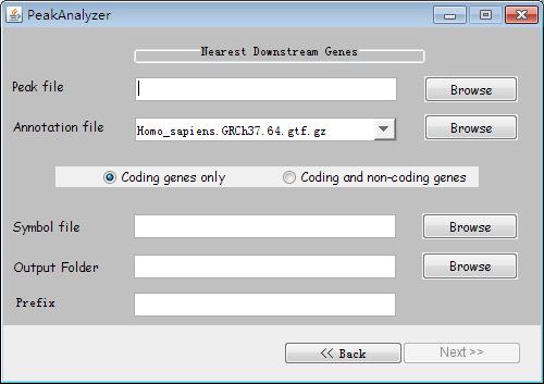
Fig. 32. The interface of Nearest Downstream Genes.
Firstly, users import the peak file by clicking the "Browse" button and select the appropriate annotation file. Then, users need to select "Coding genes only" or "Coding and non-coding genes". Afterwards, users set up the "symbol file". Subsequently, after setting the output path in "Output Folder" and typing the output file name in "Prefix". Finally, users click the button "Next" to run the program. With the progress completely, the software will give a choice for users to select whether to generate the PDF picture. Users can generate it if they have installed the R statistical software. Certainly, the results contain the information of downstream and overlapping genes in the BED format file.
We show a result file for example as below (The file name is NAME_peaks.summary.bed.):
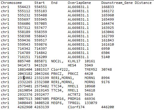
Fig. 33. An example of PeakAnalyzer result.
8.4 Obtain the gene symbols
From annotation files generated by step 3, there are a lot of columns. Users can select the annotation file by click the button "Browse". Subsequently, users click the button "Get genes" to get the gene symbols form the annotation files. Finally, users can click "Copy" button to copy the results for pathway enrichment analysis directly or "Save" to save the results in a new file.
8.5 MACS running results
The "Results" tab shows the operating state of MACS panel in ChIP-Seq analysis, such as "Begin time", "End time", "Running state" and so on.
8.6 Pathway enrichment analysis
Users can get the pathway results as shown in Chapter 5.
8.7 Pathways cross mapping
This step is same to the step 6 in chapter 6. Users can get the pathway overlapping results.
| Chapter 9 The sixth step - Meta-analysis |
The last step makes the meta-analysis of the different omics level data. Input the overlapping pathway results of three omics level and click "Cross Mapping different pathways" to generate the consistency pathway results, this leads to the final results to users.
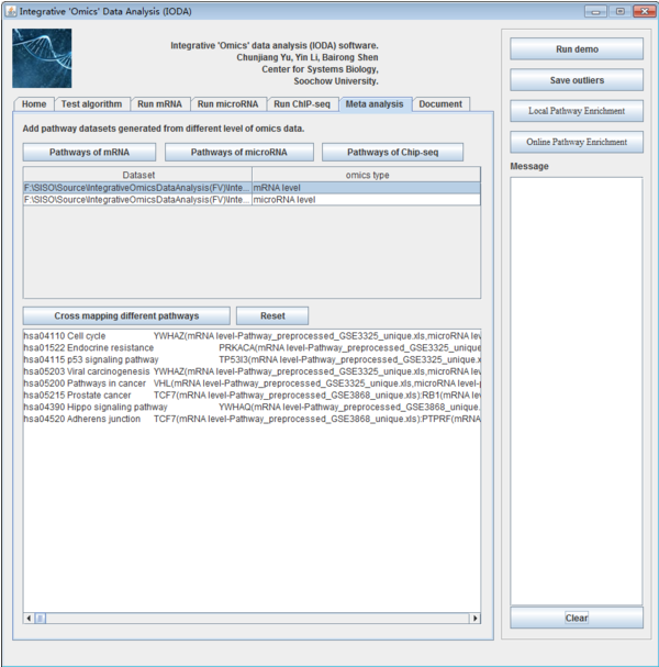
Fig. 34. The interface of Meta-analysis panel.
9.1 Input overlapped pathways of different omics level
iODA is a meta-analysis tool to analysis the data from different labs and omics data level. It can make up for the inadequacy of various datasets and show a consistency result. Users can click the different button "Pathways of mRNA", "Pathways of microRNA" and "Pathways of ChIP-Seq" to input different omics level data. After that, all the input data will be shown in the following table. The file paths are shown on the left side while the omics level of this file is shown on the right side. Users can select the datasets and then click the button "Cross mapping different pathways" and will make the consistency on these pathway results. If users click the button "Reset", the pathway list table will be clear.
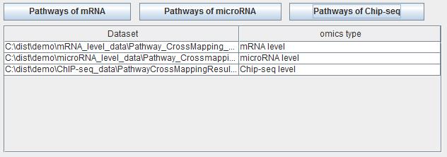
Fig. 35. The pathway list table of meta-analysis panel.
9.2 Meta-analysis process
After clicking the button "Cross mapping different pathways", the overlapping pathway results and the occurrence number will be shown in the follow textbox. And a file save dialog will show to save the consistency results.
In order to give more details of the results to the researchers, iODA provide the gene information for each pathway about this gene involved in which datasets and omics level as shown below:

Fig. 36. An example of meta-analysis result.
| Chapter 10 Run demo for iODA |
In order to show how to use iODA completely, we provide demo omics data to analysis each omics level data. All these datasets are stored in the folder "demo".
10.1 Input mRNA level omics dataset
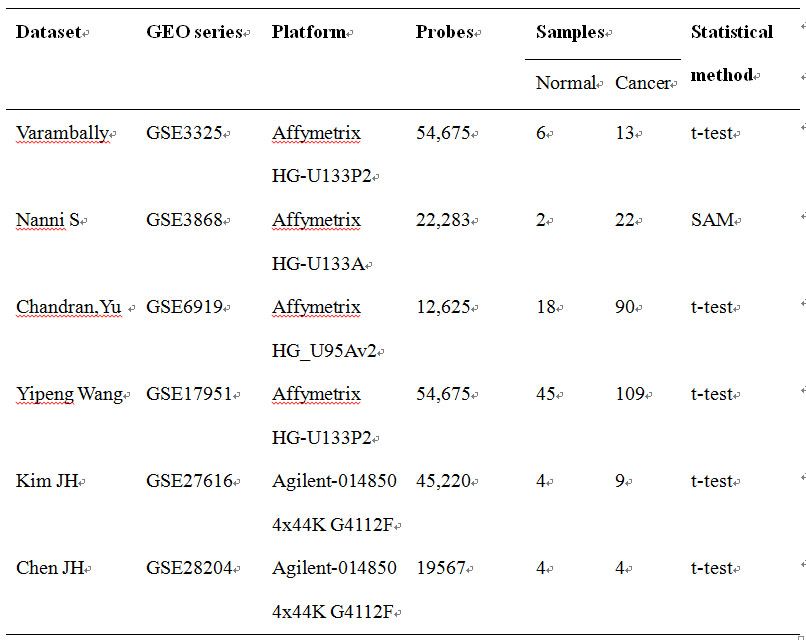
Here we provide six mRNA level microarray datasets downloaded at Gene Expression Omnibus (http://www.ncbi.nlm.nih.gov/geo/) database for prostate cancer which had been generated by independent laboratory. These datasets were measured with different technologies and platforms as shown below.
Table 3 The demo datasets of mRNA
10.2 Input microRNA level omics dataset
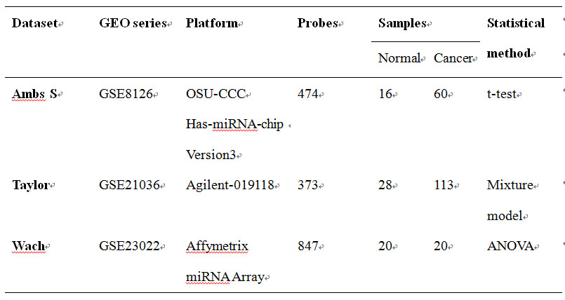
Here we provide three microarray datasets also downloaded at Gene Expression Omnibus (http://www.ncbi.nlm.nih.gov/geo/) database for prostate cancer which had been generated by independent laboratory. These datasets were measured with different technologies and platforms as shown below.
Table 4 The demo datasets of microRNA
10.3 Input ChIP-Seq level omics dataset
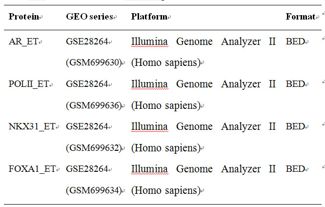
Here we provide three microarray datasets also downloaded at Gene Expression Omnibus (http://www.ncbi.nlm.nih.gov/geo/) database for prostate cancer which had been generated by independent laboratory.
Table 5 The demo datasets of ChIP-Seq
10.4 Run iODA with demo datasets
Click the button "Run demo", the demo datasets will be loaded. And the datasets will be analyzed for each dataset individually as shown below.
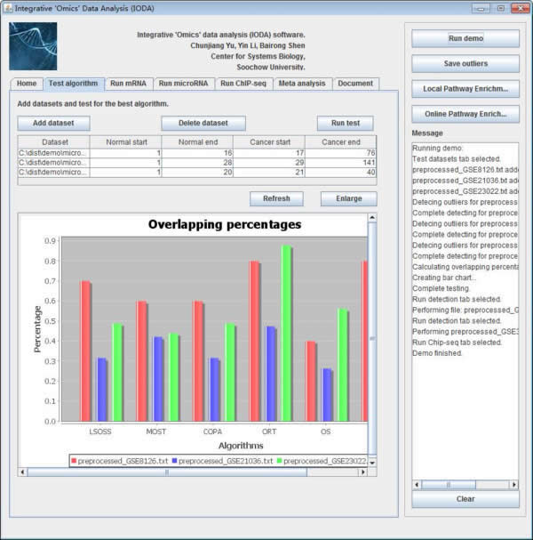
Fig. 37. The interface after click "Run demo" button.
Ashburner, M., et al. (2000) Gene ontology: tool for the unification of biology. The Gene Ontology Consortium, Nat Genet, 25, 25-29.
Bartel, D.P. (2009) MicroRNAs: target recognition and regulatory functions, Cell, 136, 215-233.
Boyle, A.P., et al. (2008) F-Seq: a feature density estimator for high-throughput sequence tags, Bioinformatics, 24, 2537-2538.
Ding, M., et al. (2012) Identification and functional annotation of genome-wide ER-regulated genes in breast cancer based on ChIP-Seq data, Comput Math Methods Med, 2012, 568950.
Fejes, A.P., et al. (2008) FindPeaks 3.1: a tool for identifying areas of enrichment from massively parallel short-read sequencing technology, Bioinformatics, 24, 1729-1730.
Ji, H., et al. (2011) Using CisGenome to analyze ChIP-chip and ChIP-Seq data, Curr Protoc Bioinformatics, Chapter 2, Unit2 13.
Kanehisa, M. and Goto, S. (2000) KEGG: kyoto encyclopedia of genes and genomes, Nucleic Acids Res, 28, 27-30.
Kozomara, A. and Griffiths-Jones, S. (2011) miRBase: integrating microRNA annotation and deep-sequencing data, Nucleic Acids Res, 39, D152-157.
Lian, H. (2008) MOST: detecting cancer differential gene expression, Biostatistics, 9, 411-418.
Lin, S.L., et al. (2010) MicroRNA miR-302 inhibits the tumorigenecity of human pluripotent stem cells by coordinate suppression of the CDK2 and CDK4/6 cell cycle pathways, Cancer Res, 70, 9473-9482.
Liu, C., et al. (2011) The microRNA miR-34a inhibits prostate cancer stem cells and metastasis by directly repressing CD44, Nat Med, 17, 211-215.
Mallick, B., Chakrabarti, J. and Ghosh, Z. (2011) MicroRNA reins in embryonic and cancer stem cells, RNA Biol, 8, 415-426.
Narlikar, L. and Jothi, R. (2012) ChIP-Seq data analysis: identification of protein-DNA binding sites with SISSRs peak-finder, Methods Mol Biol, 802, 305-322.
Redon, R., et al. (2006) Global variation in copy number in the human genome, Nature, 444, 444-454.
Tomlins, S.A., et al. (2005) Recurrent fusion of TMPRSS2 and ETS transcription factor genes in prostate cancer, Science, 310, 644-648.
Valouev, A., et al. (2008) Genome-wide analysis of transcription factor binding sites based on ChIP-Seq data, Nat Methods, 5, 829-834.
Wang, Y. and Rekaya, R. (2010) LSOSS: Detection of Cancer Outlier Differential Gene Expression, Biomark Insights, 5, 69-78.
Wu, B. (2007) Cancer outlier differential gene expression detection, Biostatistics, 8, 566-575.
Zhang, Y., et al. (2008) Model-based analysis of ChIP-Seq (MACS), Genome Biol, 9, R137. |